Table of contents
- Introduction
- Opening Phantasus
- Preparing the dataset for analysis
- Exploring the dataset
- Differential gene expression
Introduction
In this vignette we show example usage of Phantasus for analysis of public gene expression data from GEO database. It starts from loading data, normalization and filtering outliers, to doing differential gene expression analysis and downstream analysis. More detailed walk-through of the analysis is available here
To illustrate the usage of Phantasus let us consider public dataset from Gene Expression Omnibus (GEO) database GSE53986. This dataset contains data from experiments, where bone marrow derived macrophages were treated with three stimuli: LPS, IFNg and combined LPS+INFg.
Opening Phantasus
The simplest way to try Phantasus application is to go to web-site https://alserglab.wustl.edu/phantasus where the latest versions are deployed. Alternatively, Phantasus can be installed locally (see Installation).
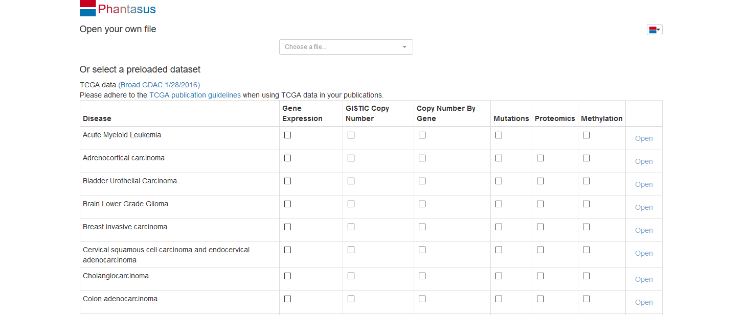
When Phantasus opens the starting screen should appear:
Preparing the dataset for analysis
Opening the dataset
Let us open the dataset. To do this, select GEO Datasets option in Choose a file… dropdown menu. There, a text field will appear where GSE53986 should be entered. Clicking the Load button (or pressing Enter on the keyboard) will start the loading. After a few seconds, the corresponding heatmap should appear.
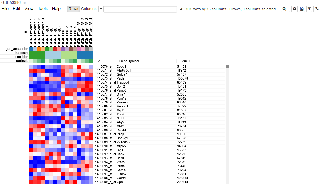
On the heatmap, the rows correspond to genes (or microarray probes). The rows are annotated with Gene symbol and Gene ID annotaions (as loaded from GEO database). Columns correspond to samples. They are annotated with titles, GEO sample accession identifiers and treatment field. The annotations, such as treatment, are loaded from user-submitted GEO annotations (they can be seen, for example, in Charateristics section at https://www.ncbi.nlm.nih.gov/geo/query/acc.cgi?acc=GSM1304836). We note that not for all of the datasets in GEO such proper annotations are supplied.
Adjusting expression values
By hovering at heatmap cell, gene expression values can be viewed. The large values there indicate that the data is not log-scaled, which is important for most types of gene expression analysis.
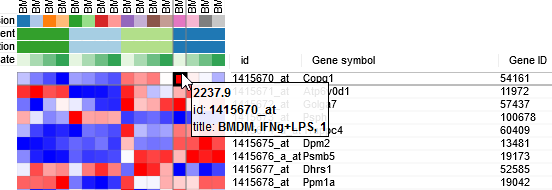
For the proper further analysis it is recommended to normalize the matrix. To normalize values go to Tools/Adjust menu and check Log 2 and Quantile normalize adjustments.
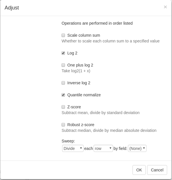
The new tab with adjusted values will appear. All operations that modify gene expression matrix (such as adjustment, subsetting and several others) create a new tab. This allows to revert the operation by going back to one of the previous tabs.
Removing duplicate genes
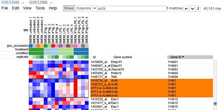
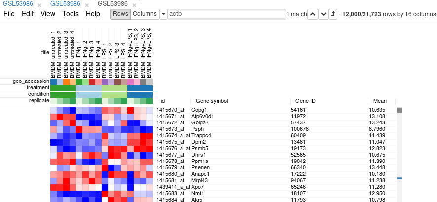
Since the dataset is obtained with a mircroarray, a single gene can be represented by several probes. This can be seen, for example, by sorting rows by Gene symbol column (one click on column header), entering Actb in the search field and going to the first match by clicking down-arrow next to the field. There are five probes corresponding to Actb gene in the considered microarray.
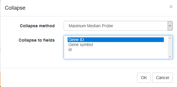
To simplify the analysis it is better to have one row per gene in the gene expression matrix. One of the easiest ways is to chose only one row that has the maximal median level of expression across all samples. Such method removes the noise of lowly-expressed probes. Go to Tools/Collapse and choose Maximum Median Probe as the method and Gene ID as the collapse field.
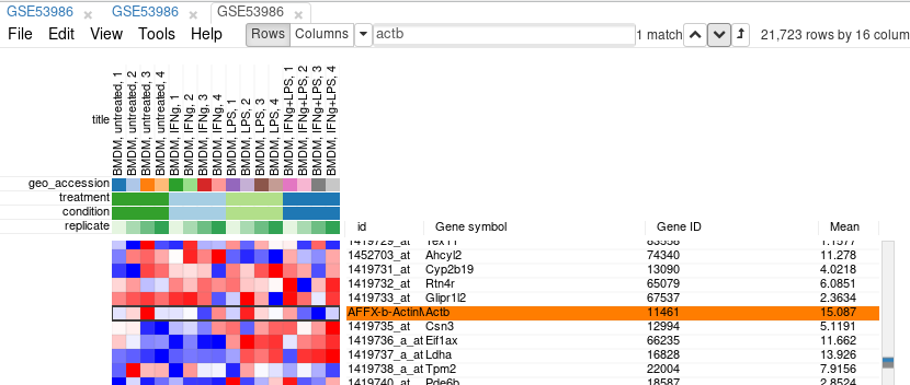
The result will be shown in a new tab.
Filtering lowly-expressed genes
Additionally, lowly-epxressed genes can be filtered explicitly. It helps to reduce noise and increase power of downstream analysis methods.
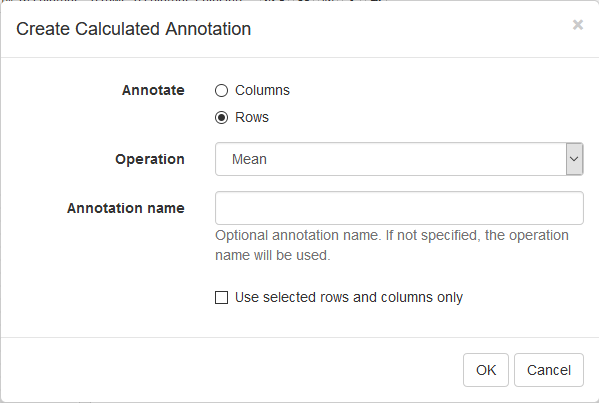
First, we calculate mean expression of each gene using Tools/Create Calculated Annotation menu. Select Mean operation, optionally enter a name for the resulting column, and click OK. The result will appear as an additional column in row annotations.
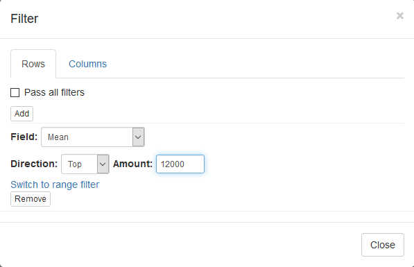
Now this annotation can be used to filter genes. Open Tools/Filter menu. Click Add to add a new filter. Choose mean_expression as a Field for filtering. Then press Switch to top filter button and input the number of genes to keep. A good choice for a typical mammalian dataset is to keep around 10–12 thousand most expressed genes. Filter is applied automatically, so after closing the dialog with Close button only the genes passing the filter will be displayed.
It is more convenient to extract these genes into a new tab. For this, select all genes (click on any gene and press Ctrl+A) and use Tools/New Heat Map menu (or press Ctrl+X).
Now you have the tab with a fully prepared dataset for the further analysis. To easily distinguish it from other tabs, you can rename it by right click on the tab and choosing Rename option. Let us rename it to GSE53986_norm.
It is also useful to save the current result to be able to return to it later. In order to save it use File/Save Dataset menu. Enter an appropriate file name (e.g. GSE53986_norm) and press OK. A file in text GCT format will be downloaded.
Exploring the dataset
PCA Plot
One of the ways to asses quality of the dataset is to use principal component analysis (PCA) method. This can be done using Tools/Plots/PCA Plot menu.
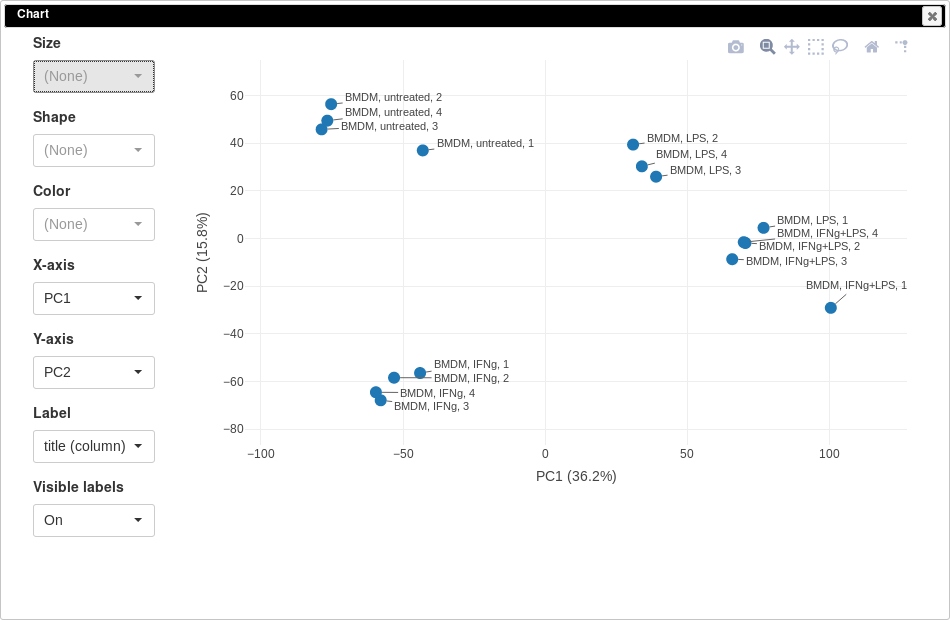
You can customize color, size and labels of points on the chart using values from annotation. Here we set color to come from treatment annotation.
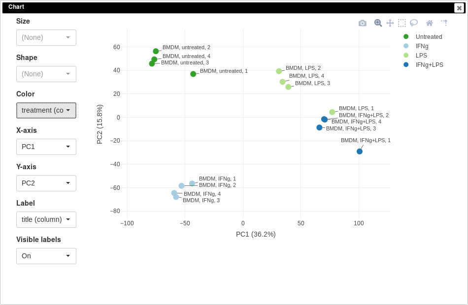
It can be seen that in this dataset the first replicates in each condition are outliers.
K-means clustering
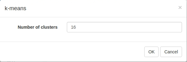
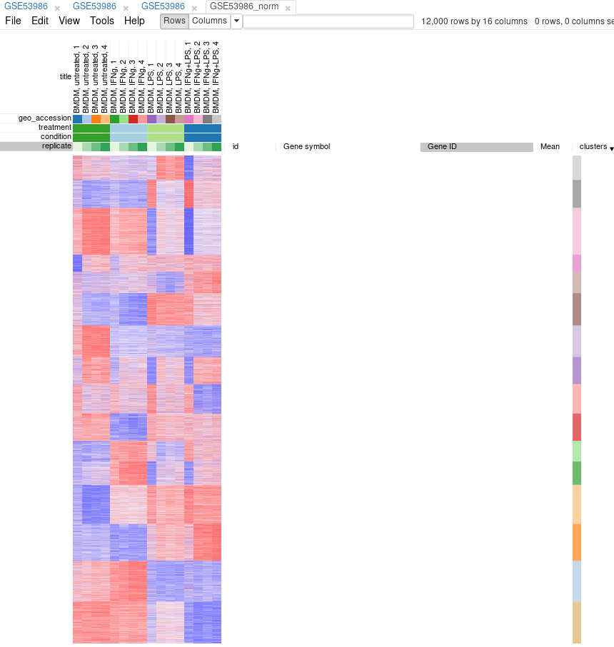
Another useful dataset exploration tool is k-means clustering. Use Tools/Clustering/k-means to cluster genes into 16 clusters.
Afterwards, rows can be sorted by clusters column. By using menu View/Fit to window one can get a “bird’s-eye view” on the dataset. Here also one can clearly see outlying samples.
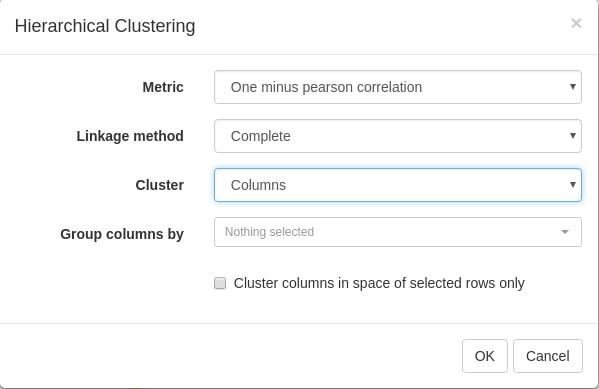
Hierarchical clustering
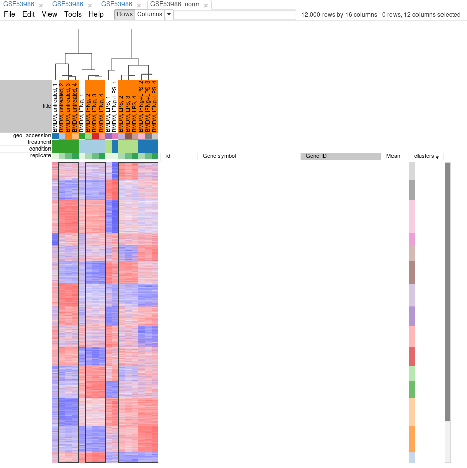
Tool/Hierarchical clustering menu can be used to cluster samples and highlight outliers (and concordance of other samples) even further.
Filtering outliers
Now, when outliers are confirmed and easily viewed with the dendrogram from the previous step, you can select the good samples and extract them into another heatmap (by clicking Tools/New Heat Map or pressing Ctrl+X).
Differential gene expression
Apllying limma tool
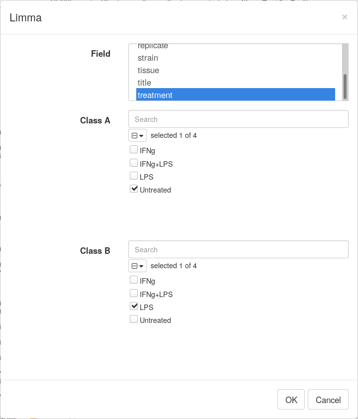
Differential gene expression analysis can be carried out with Tool/Diffential Expression/limma menu. Choose treatment as a Field, with Untreated and LPS as classes. Clicking OK will call differential gene expression analysis method with limma R package.
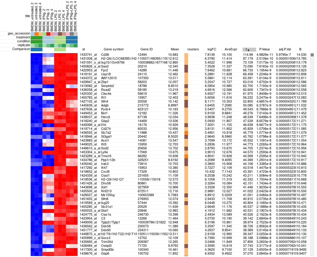
The rows can be ordered by decreasing t-statistic column to see which genes are the most up-regulated upon LPS treatment.
Pathway analysis with FGSEA
The results of differential gene expression can be used for pathway enrichment analysis with FGSEA tool.
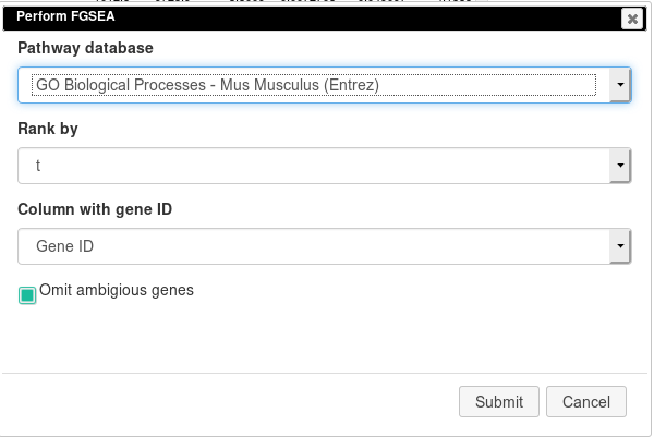
Open Tools/Pathway Analysis/Perform FGSEA, then select Pathway database, which corresponds specimen used in dataset (Mus Musculus in this example), ranking column and column with ENTREZID or Gene IDs.
Clicking OK will open new tab with pathways table.
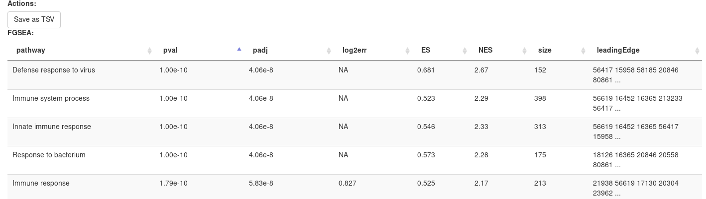
Clicking on table row will provide additional information on pathway: pathway name, genes in pathway, leading edge. You can save result of analysis in TSV format.