Table of contents
- Introduction
- Apllying limma tool
- Saving and sharing the results
- Pathway enrichment with MSigDB
- Visualizing pathway enrichment
- Pathway enrichment with FGSEA
- Other tools for pathway analysis
Introduction
This is the third of three related modules:
In this module we start with a normalized and filtered dataset, do a differential expression analysis and follow it up with pathway enrichment analysis.
You can either continue the session from the previous module, or download file GSE53986_filtered.gct and load it into Phantasus.
Apllying limma tool
Differential expression analysis is one of the most straightforward types of analysis to carry out on gene expression data. It answers a question what genes a differentially regulated between two conditions of interest.
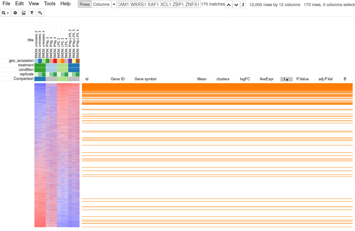
After dataset is properly normalized limma R package can be used to do differential expression analysis. Open Tool/Diffential Expression/limma menu, Choose treatment as a Field, with Untreated and LPS as classes.
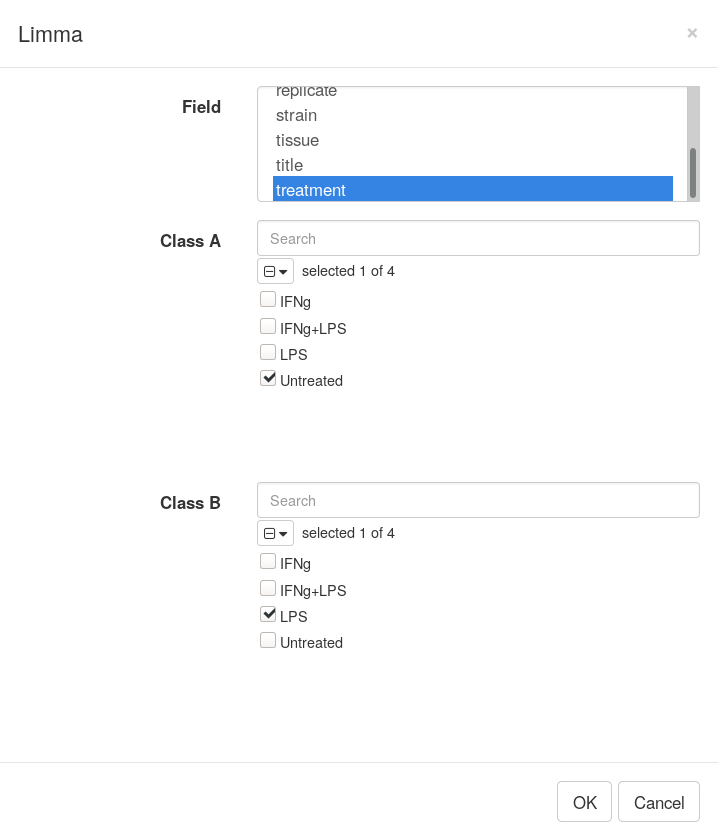
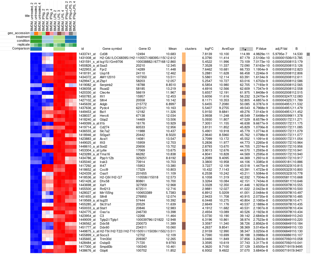
Clicking OK will add columns like P-value or logFC to the table. The rows can be ordered by decreasing of t-statistic column to see which genes are the most up-regulated upon LPS treatment.
Saving and sharing the results
We have found genes differentially regulated upon LPS treatment. Now we can save the results as a GCT file to able to return to it later or share with a colleague. The resulting file should be similar to GSE53986_Ctrl_vs_LPS.gct.
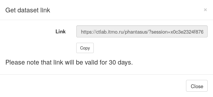
However, in Phantasus you can share the result by providing link to the current session. Use File/Get dataset link menu. After you click on it, a window will appear containing a link, that you can share with other people. Accessing it will load an identical session.
Pathway enrichment with MSigDB
While we now know what genes are differentially regulated between our two conditions of interest, these results can be hard to interpret. There can be too many or too few differential genes, a gene can multiple functions and so on. Naturally, it is much easer to reason about biological processes, or pathways. A pathway has many genes, which makes its signal to be more robust and it has a particular function.
There are many ways to analyze pathways, with over-representation analysis being one of the most straightforward. In this analysis we will have a query gene set, such as top 250 up-regulated genes, and we will be looking for biological pathways that have a big intersection with our query. For such pathways we can speculate that they are regulated in our process as well.
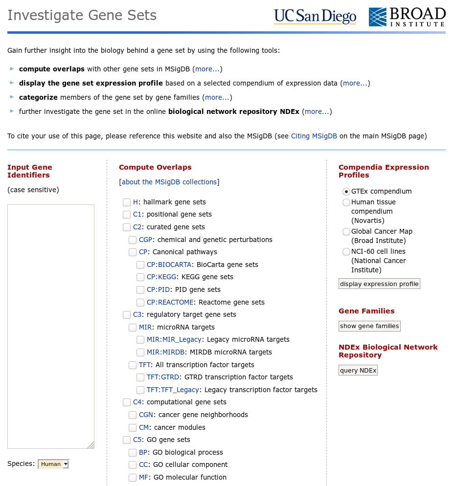
Let us open a MSigDB web tool for such analysis: http://software.broadinstitute.org/gsea/msigdb/annotate.jsp. MsigDb requires registration but it is free. After logging in “Investigate Gene Sets” window should appear.
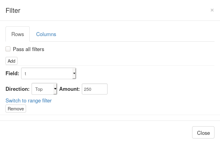
Now let us go back to Phantasus where we will be selecting top 250 up-regulated genes. For this we will us Tools/Filter menu. There add a top filter by t column for 250 genes.
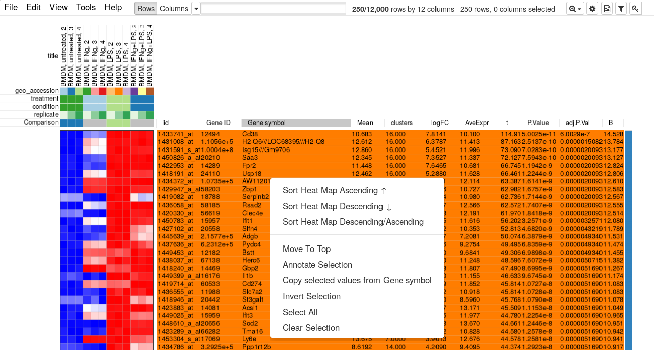
Next close the filter window and select all of the displayed genes. To copy gene symbol do a right-click on any value in Gene symbol column and select Copy selected values from Gene symbol option. After copying go back to Tools/Filter menu and remove the filter, so that all 12000 genes are displayed again.
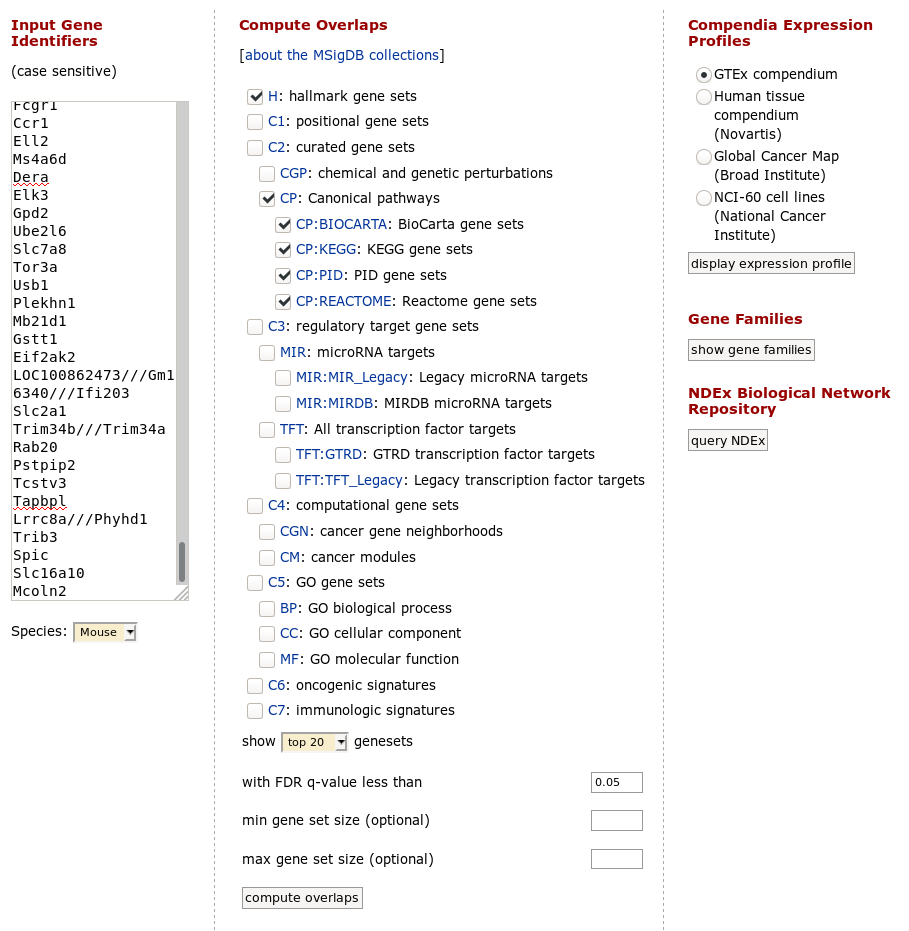
Paste the copied gene symbols to MSigDB, select proper species (mouse) and select H: hallmark gene sets and CP: Canonical pathways collections. Also, you can change parameters to show top 20 gene sets. Click on compute overlaps to run the analysis.
The screen features some statistics and the table with pathway p-values. All the top pathways are immune singling pathways, in particular interferon response, which is not unexpected. However, in normal analysis, where the biology is not that well-known, such analysis proves to be very useful.
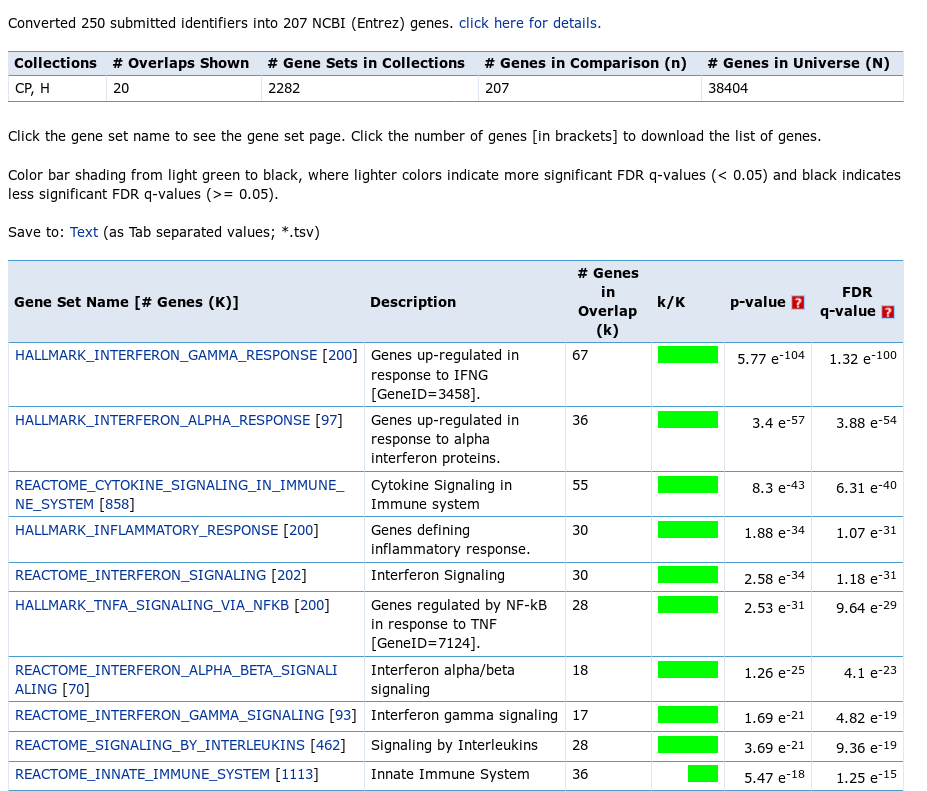
There is one important moment that should be considered, when MSigDB analysis is executed. MSigDB web tool uses hypergeometric test as a statistical measure of overlap significance. An essential parameter of the test is the background gene set (also called “universe”), from which the query genes were selected. In the reported statistics you can see that for the test a universe of 38404 genes has been used, however the query was constructed by selecting from only 12000 genes. This discrepancy leads to overreported results and the real p-values are less significant than the reported ones. Pathways with very low reported q-value, such as 1e-12, won’t become non-significant after the correction, but pathways with q-value on the order of 1e-3–1e-4 should be taken with caution.
Visualizing pathway enrichment
A common way to visualize enrichment of individual pathways is to use GSEA (gene set enrichment analysis) plot. In our case let consider Interferon Gamma Response pathway.
First, go to the pathway description: http://www.gsea-msigdb.org/gsea/msigdb/cards/HALLMARK_INTERFERON_GAMMA_RESPONSE.html. There, click on text format in Download gene set row, which will get you a file with a list of genes in this pathway: geneset.txt.
Copy the genes from the pathway and paste them in search field in Phantasus. Sort the dataset by t column and select Fit To Windows zoom option to get an overview of how the whole pathway is regulated. You will be able to see that not just the top 250 up-regulated genes contain many Interferon Gamma Response pathway genes, but overall the genes from this pathway tend to be in the upper part.
To quantify and better show the up-regulation trend GSEA analysis and GSEA plot can be used. Go to Tools/Plot/GSEA plot. In the tool option select t column for ranking and select condition for annotation. This will result in the following plot.
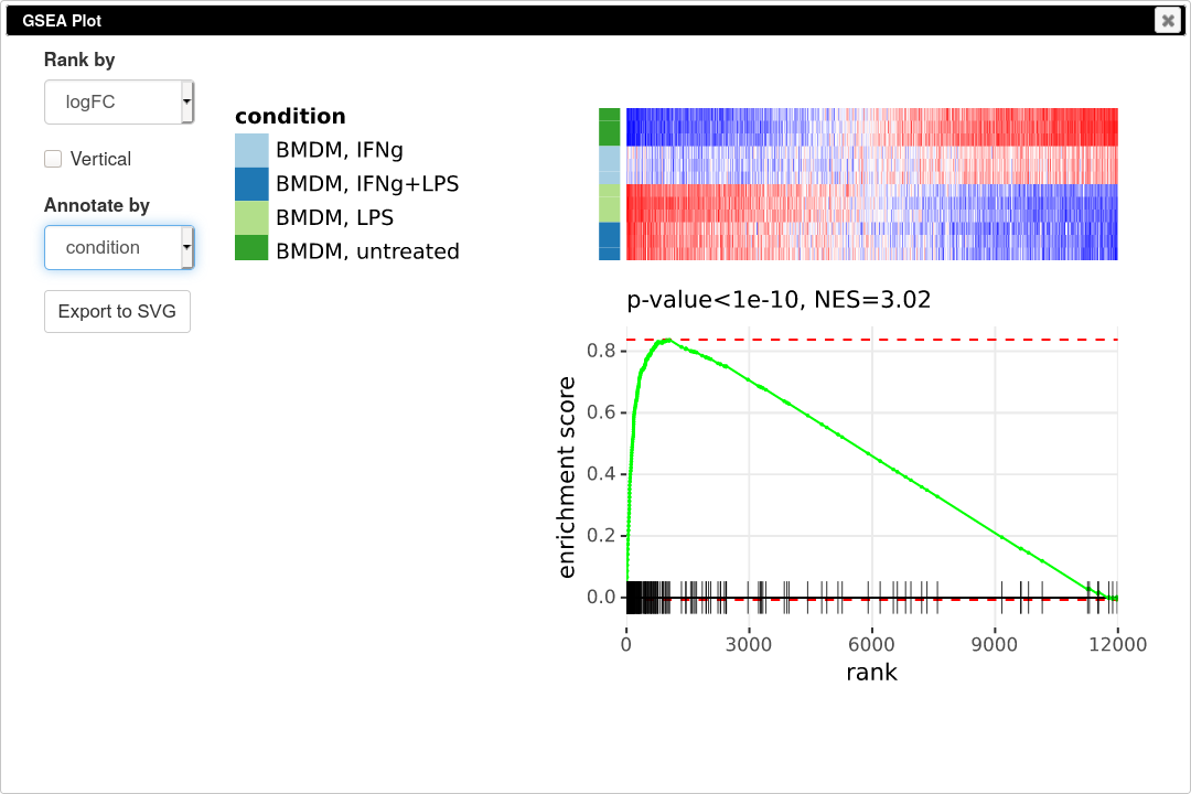
GSEA plot works as follows. First, the genes are ordered according to some metric, such as t-statistic that we used. Next the genes are traversed one by one and if the gene is present in the considered pathway the curve goes up, and it goes down otherwise. If the genes of the pathway tend to be up-regulated, as in our case, the curve will first go up and then go down. If the pathway is down-regulated, the genes will be shifted towards the other end and the curve will first go down and then up. If the pathway is not regulated at all, then genes will be approximately uniformly distributed in the ranking and the curve will also represent a random walk without any specific trend. The displayed P-value shows quantitatively the non-randomness of the behavior. An important aspect of GSEA analysis is that it does not require selecting any threshold, unlike hypergeometric based analysis described in the previous section.
Pathway enrichment with FGSEA
GSEA analysis can be also carried systematically for a collection of pathways with FGSEA tool.
Open Tools/Pathway Analysis/Perform FGSEA, then select Pathway database, which corresponds specimen used in dataset (Mus Musculus in this example), ranking column and column with ENTREZID or Gene IDs.
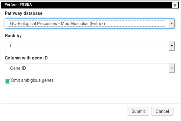
Clicking OK will open new tab with pathways table.
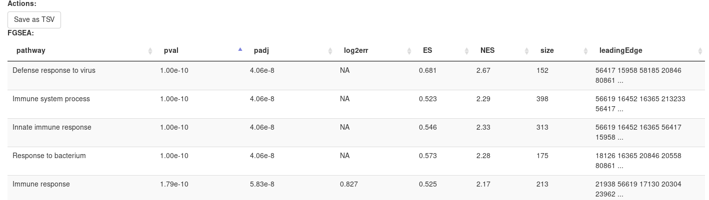
Clicking on table row will provide additional information on pathway: pathway name, genes in pathway, leading edge. You can save result of analysis in TSV format.
Other tools for pathway analysis
Aside mention above tools for pathway enrichment analysis there are few more sometimes more suitable tools:
- Enrichr feature many diverse pathway collections, especially interesting is transcription regulation collections. As Enrichr is strict to its input, Tools/Pathway analysis/Submit to Enrichr menu can be used to simplify access.
- WebGestalt can do pathway analysis for many organisms. Additionally, the background gene set can be specified for over-representation analysis, which make results much more accurate.
- GeneQuery can be used to search for signatures among public datasets from Gene Expression Omnibus.