Table of contents
- Introduction
- Obtaining Gene Expression Omnibus entry
- Basic controls
- Data normalization
- From probes to genes
- Saving and loading datasets in gct
Introduction
This is the first of three related modules:
In this module we cover steps from finding a gene expression dataset link in a published paper to a normalized dataset, prepared for exploration and further analysis.
Obtaining Gene Expression Omnibus entry
Let’s start from a most common unit of scientific knowledge: a publication. Imagine, you found a nice paper which mentions gene expression analysis by microarray, for example this one. Thankfully most journals nowadays require the gene expression data deposited publicly, which means that we can look more closely at the data, beyond what is described in the original publication.

The dataset link usually resides either in dedicated data availability statement, or in methods section as in this case. We are looking for something like “accession number” followed by an identifier. Here we have “GSE53986”. There can be different kinds of identifiers, but in this tutorial we focus on the GSEnnnnn ones.

The easiest way to go to the corresponding database entry is just use Google. The first link would be https://www.ncbi.nlm.nih.gov/geo/query/acc.cgi?acc=GSE53986, which is exactly what we need.
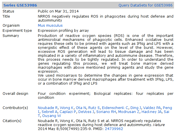
The entry contains basic information like title of the dataset, abstract, link to the publication and so on. From the samples list we can easily see that the dataset contains four biological conditions: control bone-marrow derived macrophages (BMDMs) and BMDMs activated with either LPS, interferon-gamma or both of them simultaneously.
Basic controls
Now let us open the dataset in Phantasus. Use https://alserglab.wustl.edu/phantasus mirror. Then click on Choose a file input, select GEO Datasets, enter GSE53986 and click Load button (or press Enter on the keyboard).

After the dataset is loaded you will see the heatmap interface. The heatmap columns correspond to the 16 biological samples in this experiment. The rows correspond genes (or, more accurately, to microarray probes). If you hover the mouse cursor over a cell a pop-up will appear displaying the expression value of the corresponding gene in the corresponding sample. By default a row-relative scheme is used: blue color corresponds to the lowest expression in a row and red color corresponds to the highest one.

Besides expression values the annotation for genes (Gene ID, Gene symbol) and samples (treatment, condition) are displayed. The annotations are loaded from user-submitted GEO annotations (they can be seen, for example, in Charateristics section at https://www.ncbi.nlm.nih.gov/geo/query/acc.cgi?acc=GSM1304836). We note that not for all of the datasets in GEO such proper annotations are supplied. Additionally condition and replicate annotations are generated automatically based on sample names.
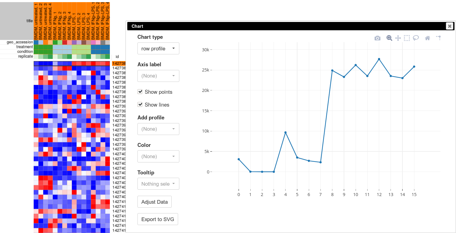
When opening a new dataset it’s usually helpful to check marker genes to confirm that the dataset is what you expect it to be. Here let’s check known marker of macrophage activation: Acod1. Put the gene name into the search field and click down arrow to scroll to the hit. We can see, that the gene is highly up-regulated in LPS and LPS+IFNg conditions.

If you look at the expression values more closely you will be able to see that there is some up-regulation of Acod1 in IFNg. That can be more easily seen if we plot the expression using Tools/Plots/Charts. Select all the columns to show the values in all the samples.
Data normalization
Importantly the gene expression values are better to consider in logarithmic scale in most cases. There are two related reasons for this. First, the fold-changes are more interpretable: if we see an mRNA two-fold change it’s probably important, independent of the actual base-level concentrations. Second, many statistical models assume that the noise is normally-distributed, which is much more the case in log-scaled expression than in the linear scale.
Sometimes the gene expression data can be already log-scaled, some time it is not. The simplest way to check it is to look at the expression values. If they are small (say, in the range 0–20), then the data is already scaled, if there are big number (say, greater then 100), then the data is in linear scale.
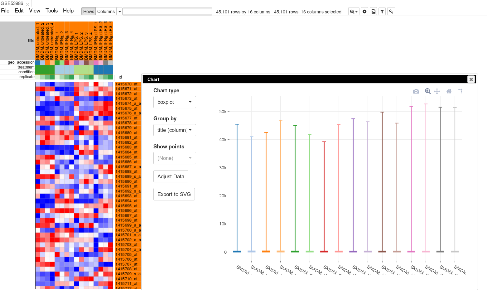
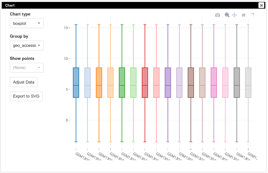
The more accurate way to check scale is to get a box-plot of all the expression values in in the sample. Select all the genes and all the samples. Open Tools/Plots/Charts dialog, select boxplot in Chart type. Select title (column) in Group by to show the boxplots by sample. From the plot you can clearly see that there is a wide range of expression values.
To apply log-scale normalization go to Tools/Adjust menu, check Log 2 and click OK. A new tab with log scaled values will appear: all operations that modify gene expression matrix create a new tab, which allows to revert the operation by going back to one of the previous tabs. If we do a boxplot again, we will see that the range of the expression values is much smaller now, and it is more symmetrical.
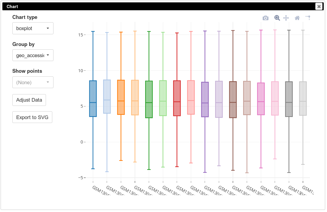
On the same plot you can see some variation of expression distribution between the samples. For example, the second sample seems to have overall higher expression values compared to the first one. This can happen for multiple reasons, in particular there can be just more input mRNA.
To be able to better compare different samples we will normalize distributions using so-called quantile normalization. This can be done using Tools/Adjust menu and checking Quantile normalize option. After that, again, a new tab will appear with normalized values. If we plot the distribution using boxplots, we will see that the distributions are now identical.
Few remarks about the normalization:
- Log-scale and quantile normalization can be done in one step by checking both checkboxes simultaneously.
- Check that you haven’t done log-scale twice: if the range of values becomes around 0–4 that’s probably what happened.
- Quantile normalization can usually won’t make anything worse, so if you are not sure whether some inter-sample normalization was applied, it is usually safe to apply quantile normalization just in case.
From probes to genes
If you have looked some other genes in the table you could have noticed that some of the genes are present in the table multiple times. Indeed, in microarrays oligonucleotide abundance, not gene one, is measured and multiple oligonucleotides can match to a single gene, as well as one oligonucleotide sequence can be present in multiple genes.
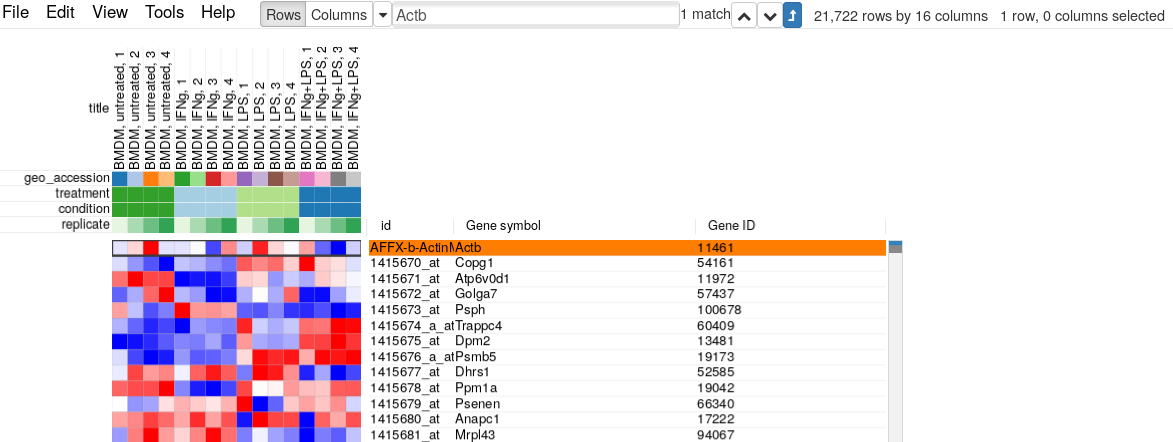
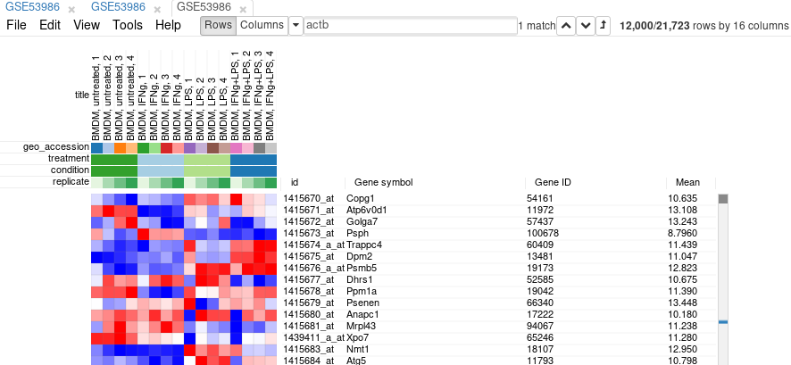
For example, let’s put Actb gene in the search field and click “Matches to top” button. We can see that there are five microarray probes mapped to Actb gene.

It is usually much more convenient in terms of analysis and interpretation to work with gene-level, not probe-level, expression values. This requires a collapse procedure to go from multiple gene entries to a single entry.
There are multiple ways of collapsing. Probably, the most naive way is just to average expression of a gene among all the corresponding probes. However, there can be very noisy probes, which we would rather throw out, and not spoil the other values.
The other way which we usually recommend is to select the probe with the highest average expression level. This has two advantages:
- usually the noisy probes are the ones with low expression (exercise: plot probe profiles for Actb and check that the lowest probe indeed has the most variance), and
- we can trace gene expression to a particular measurement which can help if there are problems downstream.
To collapse probe to genes we will use Tools/Collapse menu. We mentioned before we will be keeping only the highest expressed probe for a gene. In this case it will be measured by median expression (in log-scale, the mean expression can be used as well), so select Maximum Median Probe as a collapse method. Selecting Gene ID in Collapse to fields will group the probes based on Gene ID field and will ensure that after collapse there are no duplicate entries in Gene ID column.

The resulting table will contain only 21722 rows (which is equal to approximate 20K protein-coding mouse genes) with only one entry for Actb gene, coming from probe “AFFX-b-ActinMur/M12481_3_at”:
Finally, it is useful to get rid of unexpressed or lowly expressed genes to decrease noise amount in our data. It is particularly important for microarrays, where even for absent genes there will be non-zero values due to cross-fluorescence.
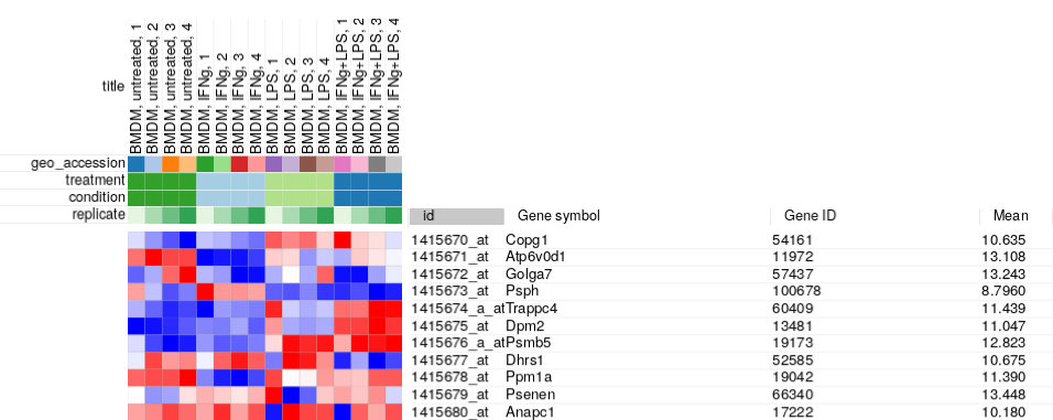
An easy way to do it in Phantasus is to filter genes based on average expression. First for each gene we obtain average values using Tools/Create Calculated Annotation menu:

After clicking OK a new column with average values should appear:
To filter the genes we will be using Tools/Filter menu. Click Add to add a new filter. Choose Mean as a Field for filtering. Then press Switch to top filter button and input the number of genes to keep. A good choice for a typical mammalian dataset is to keep around 10–12 thousand most expressed genes. Another option to filter is to use a strict threshold with a range filter, but this requires selection of an appropriate threshold which depends on a dataset, so a top filter is much more convenient.
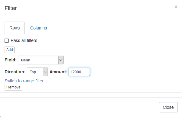
Filter is applied automatically, so after closing the dialog with Close button only the genes passing the filter will be displayed.
It is more convenient to extract these genes into a new tab. For this, select all genes (click on any gene and press Ctrl+A) and use Tools/New Heat Map menu (or press Ctrl+X).
Saving and loading datasets in gct
The resulting dataset can be saved locally, so that it can be easily reloaded. In order to save it use File/Save Dataset menu. Enter an appropriate file name (e.g. GSE53986_norm) and press OK.

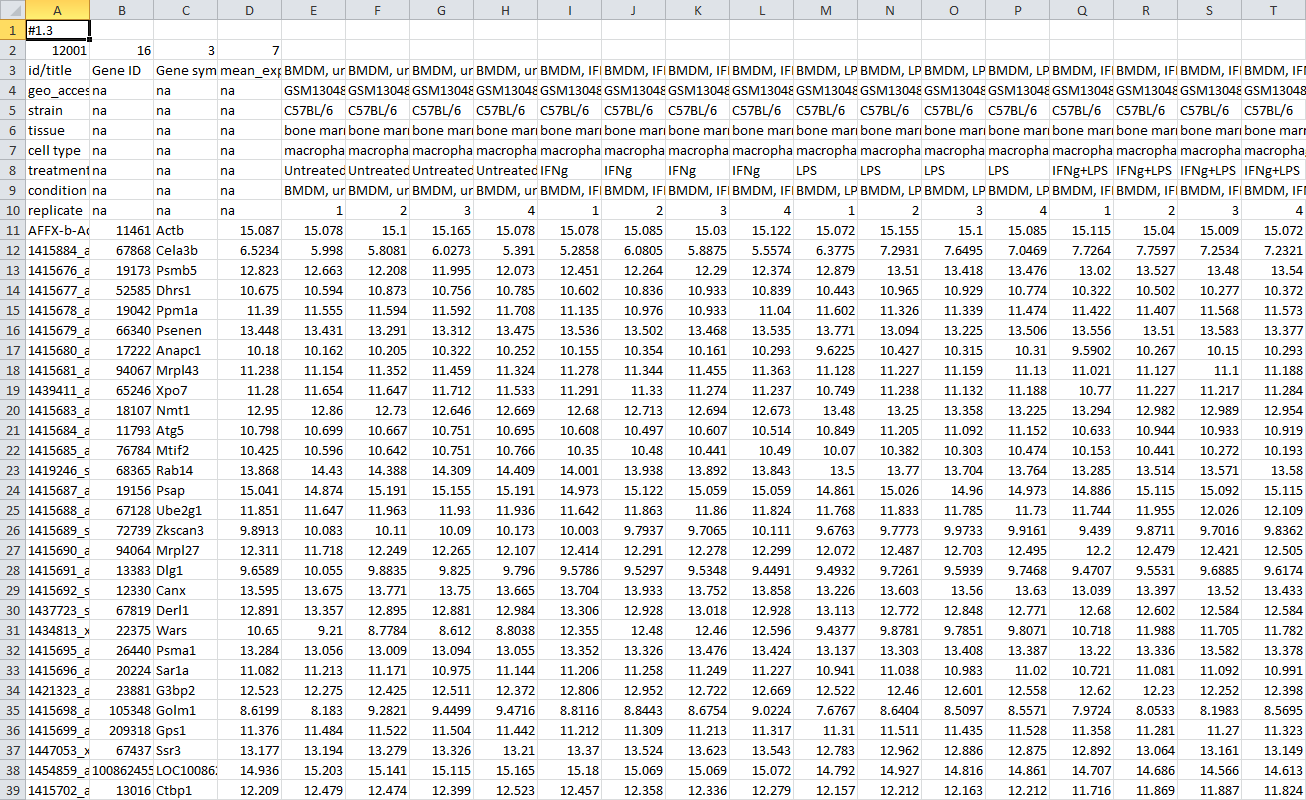
After that a file in a text GCT format will be downloaded. The file should be similar to GSE53986_norm.gct. As GCT is a text format, you can open and modify it in a text or spreadsheet editor.
To load dataset use File/Open menu, click on Open your own file dropdown menu, click on My computer and select there the gct file. The file will be opened in a new tab. Similarly, a file can be opened from the home screen.